
ETL 1110-2-563
30 Sep 04
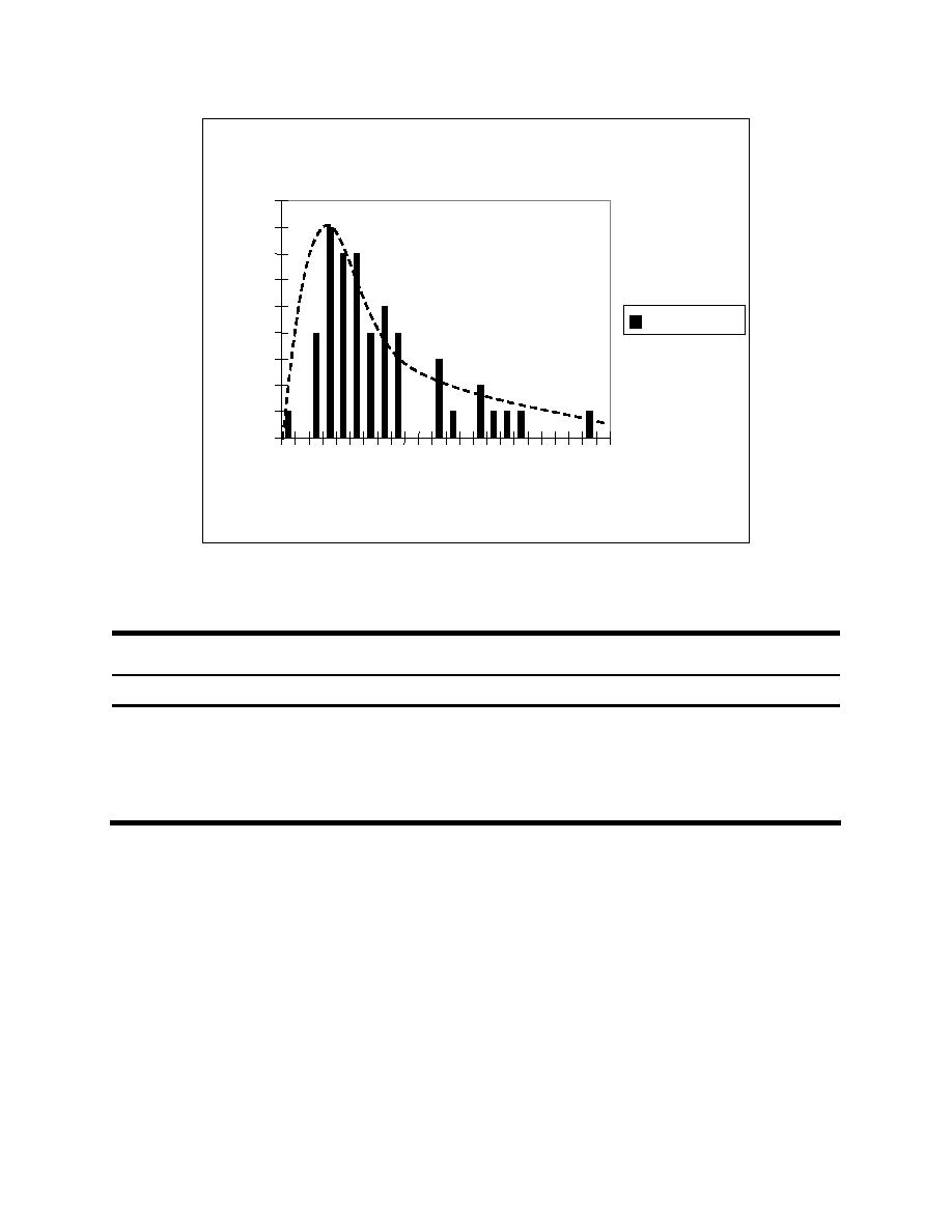
Fitted Distribution for Angles
Lognormal (3.86, 2.31)
9
8
7
6
5
4
3
2
1
0
2 3.5
5 6.5
8 9.5
11
0.5
Angle (degrees)
Figure D-7. Histogram of impact angle from experiments (note: lognormal
distribution is fitted dashed line)
Table D-3
Fitted Distributions for Scale Model Data
Standard
Distribution Type
Mean
Deviation
Truncation
Longitudinal
Lognormal
0.439 m/sec
1.67 m/sec
2 m/sec (6 ft/sec)
x-velocity
(1.44 ft/sec)
(5.5 ft/sec)
Transverse
Lognormal
0.0146 m/sec
0.026 m/sec
0.3 m/sec (1 ft/sec)
y-velocity
(0.048 ft/sec)
(0.083 ft/sec)
Angle (degrees)
Lognormal
1.176 m/sec
0.704 m/sec
None
(3.86 ft/sec)
(2.31 ft/sec)
(5) The spreadsheet developed for this example uses the empirical equation discussed in para-
graph B-3 of this ETL. The data input to the cells for this example are shown in Figure D-8. @Risk uses
the calls of "RiskLognorm" within a cell to define the lognormal random variable with its mean and
standard deviation. The "RiskTruncate" command limits the sampling of the distribution above those
values. The output for Fm uses the "RiskOutput" command and the empirical equation follows the name.
Uncertainty in the empirical model is not included in this example for simplicity. Based on the processing
of the data to define the empirical equation as discussed in Appendix E, the standard deviation (or error)
in the empirical model is 351 kN (79 kips). This would need to be included in the PBIA as approxi-
mately a 10 percent coefficient of variation during the simulation of impact force results. These varia-
tions of the model would be represented by a cone shape running from 0 to 800 kips, which is shown in
Appendix E, Figure E-3. These values input to the spreadsheet cells reflect the values from Table D-3.
D-7

 Previous Page
