ETL 1110-2-547
30 Sep 95
and FY = Fln X. To obtain the parameters of the normal
assumed probability density function. It is defined in
terms of the mean X and standard deviation FX as:
random variable Y, first the coefficient of variation of
X is calculated:
x&
2
FX
1
fX X '
exp &
VX '
2 F2
F 2B
EX
The standard deviation of Y is then calculated as:
When fitting the normal distribution, the mean of the
distribution is taken as the expected value of the
random variable. The cumulative distribution function
FY ' Fln X '
2
ln 1 % VX
for the normal distribution is not conveniently ex-
pressed in closed form but is widely tabulated and can
The standard deviation FY is in turn used to calculate
be readily computed by numerical approximation. It is
the expected value of Y:
a built-in function in most spreadsheet programs.
Although the normal distribution has limits of plus and
F2
minus infinity, values more than three or four standard
Y
E Y ' E ln X ' ln E X &
deviations from the mean have very low probability.
2
Hence, one empirical fitting method is to take
minimum and maximum reasonable values to be at
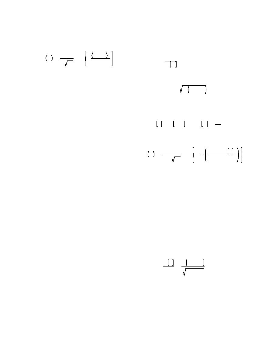
The density function of the lognormal variate X is:
plus and minus three or so standard deviations. The
normal distribution is commonly assumed to
ln X & E Y
characterize many random variables where the
2
1
1
fX '
exp &
coefficient of variation is less than about 30 percent.
FY
X FY
2B
2
For levees, these include soil density and drained
friction angle. Where the mean and standard deviation
are the only information known, it can be shown that
The shape of the distribution can be plotted from the
the normal distribution is the most unbiased choice.
above equation. Values on the cumulative distribution
function for X can be determined from the cumulative
d. Lognormal distribution.
distribution function of Y (E[Y], FY) by substituting the
X in the expression Y = ln X.
(1) When a random variable X is lognormally
distributed, its natural logarithm, ln X, is normally
distributed. The lognormal distribution has several
B-7. Calculation of the Reliability Index
properties which often favor its selection to model
certain random variables in engineering analysis:
a. Figure B-2 illustrates that a simple definition
of the reliability index is based on the assumption that
As X is positive for any value of ln X,
capacity and demand are normally distributed and the
lognormally distributed random variables
limit state is the event that their difference, the safety
cannot assume values below zero.
margin S, is zero. The random variable S is then also
normally distributed and the reliability index is the
It often provides a reasonable shape in cases
distance by which E[S] exceeds zero in units of FS:
where the coefficient of variation is large
(>30 percent) or the random variable may
ES
EC&D
$'
'
assume values over one or more orders of
FS
F2 % F2
C
D
The central limit theorem implies that the
An alternative formulation (also shown in Figure B-2)
distribution of products or ratios of random
implies that capacity C and demand D are lognormally
variables approaches the lognormal distri-
distributed random variables. In this case ln C and ln
bution as the number of random variables
D are normally distributed. Defining the factor of
increases.
safety FS as the ratio C/D, then ln FS = (ln C) - (ln
D) and ln FS is normally distributed. Defining the
(2) If the random variable X is lognormally
reliability index as the distance by which ln FS
distributed, then the random variable Y = ln X is
normally distributed with parameters E[Y] = E[ln X]
B-6


 Previous Page
